The Chaos Labs Uniswap V3 LP Simulation platform is a publicly accessible tool expressly tailored to facilitate market makers in making astute decisions regarding asset and strategy selection. This is achieved by curating a user-friendly interface that provides optimal matches based on user preferences and a comprehensive analysis of the simulation results.
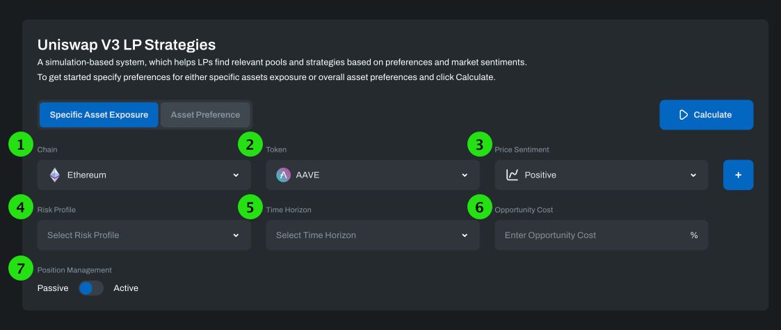
Blockchain Preference
The Uni V3 Backtester is compatible with Uniswap V3 deployments on Ethereum and Polygon networks.
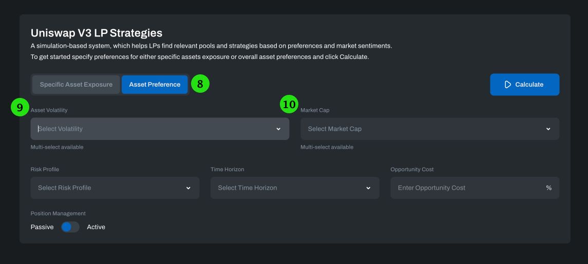
(2) Asset Preference
The user is tasked with selecting the token for which they wish to provide liquidity. In contrast to other platforms, which necessitate explicit pool selection, the Uni V3 backtester employs a more user-centric approach. It autonomously scans high-volume pools containing the selected token, opting for only the most relevant pools.
(3) Price Sentiment Analysis
Users are invited to provide their estimation of the price sentiment for the selected asset. They have the autonomy to select the market type they wish to apply for data simulation. The available choices align with positive, neutral, or negative market sentiments:
- Positive - the market maker anticipates an upsurge in the asset price
- Neutral - the market maker foresees the asset price to stabilize around current levels
- Negative - the market maker predicts a downturn in the asset price
Price sentiment enables users to express a broad perspective on an asset's price movement rather than indicating a precise rate of price alteration.
When opting for a positive price sentiment, the historical testing interval will correspond to the week or month exhibiting the most substantial price increase within the preceding 180 days.
Conversely, when selecting positive price sentiment, the backtesting timeframe will align with the week or month featuring the most significant price decline over the preceding 180 days.
In the event of a positive price sentiment selection, the backtested period will align with the week or month, displaying the slightest price variation throughout the last 180 days.
(4) Risk Tolerance Assessment
Users are required to delineate their risk tolerance level. In line with standard financial investment principles, the potential for profit escalates with risk. The selectable options range from conservative, through aggressive, to very aggressive. Typically, users selecting a higher-risk profile will opt for a narrower range of liquidity provisions. Moreover, those with a higher risk tolerance are more likely to dedicate more time to liquidity provisioning than their conservative counterparts.
(5) Investment Duration
Users are afforded the opportunity to select an investment duration from a range of pre-defined time frames, including 1 Week and 1 Month.
(6) Alternative Cost Analysis
Users are guided to specify their alternative cost to LPing. For instance, if they borrow funds for the purpose of providing liquidity, this would be the Annual Percentage Rate (APR) of the loan. This data is then employed to calculate their Profit and Loss (PnL) statement.
(7) Position Management
The Uni V3 Backtester caters to diverse user proficiencies by offering passive and active strategy evaluation. With passive strategies, liquidity is supplied within a specified range throughout the entire backtesting duration. This approach best suits users who do not leverage automated systems to oversee their positions. On the other hand, more advanced users may opt for active strategies. Here, liquidity is strategically withdrawn and redeployed in response to market price alterations. Further insights into these distinct strategies can be garnered from the Market Making Strategies section above.
The Chaos Labs Uni V3 Backtester offers a comprehensive view of the most profitable pools and strategies tailored to users’ preferences. Users can evaluate different options based on specific pool composition, PnL, as well as alternative costs of LvR and the rebalancing frequency.
(9) Asset Volatility Analysis
In the backtesting process, the assets are classified into three distinct groups according to their historical volatility. Users can express a preference for the volatility level of the assets they wish to provide liquidity.
(10) Market Capitalization and Type Assessment
Another salient factor that market makers often consider when differentiating between assets is their market capitalization. Users are thus given the flexibility to select either higher or lower market cap tokens for liquidity provision. This functionality enriches the Chaos Labs Uni V3 Backtester's customization potential, empowering users to tailor their investment strategy to their unique objectives and risk tolerance.
Although stablecoins can have varying market cap levels, the nature of market-making in pools where both assets are stablecoins is different due to their low price volatility and high concentration of liquidity. As a result, users can explicitly choose to make markets in those pools.
Blue Chip BTC, ETH High Market Cap >$1B Medium $250M < Market Cap < $1B Stables Pool Pools where both assets are stablecoins
| Type | Market Capitalization |
|---|---|
| Blue Chip | BTC, ETH |
| High | Market Cap >$1B |
| Medium | $250M < Market Cap < $1B |
| Stables Pool | Pools where both assets are stablecoins |
LP Backtesting Simulation Results
The Chaos Labs Uni V3 Backtester offers a comprehensive view of the most profitable pools and strategies tailored to users’ preferences. Users can evaluate different options based on specific pool composition, PnL, as well as alternative costs of LvR and the rebalancing frequency.
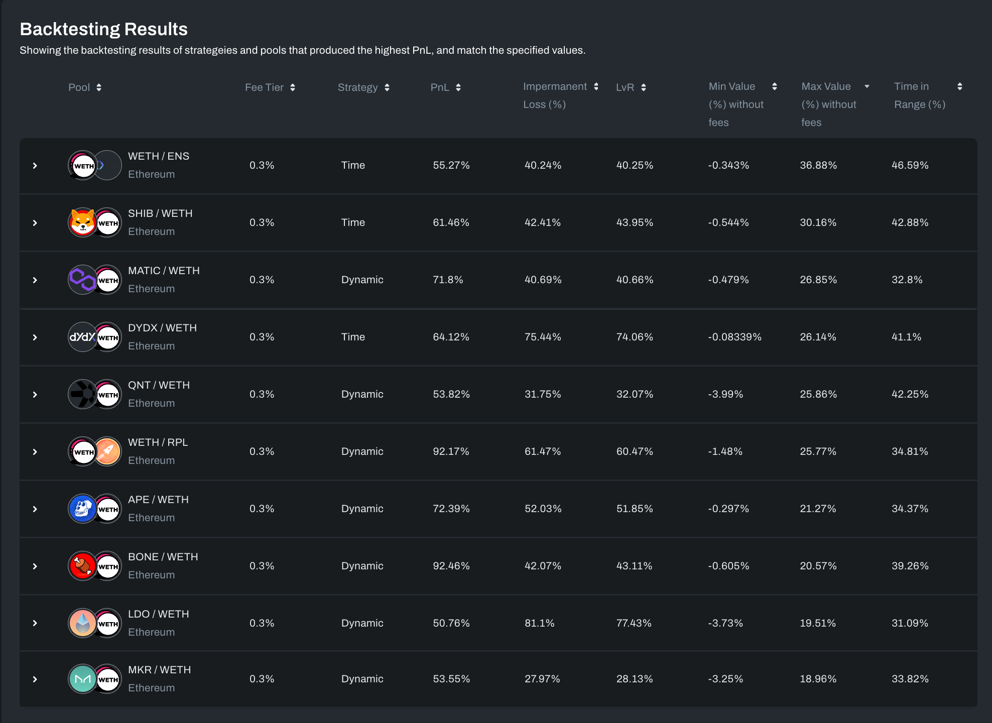
LP Strategy Backtest Drill-Down
The potency of the Chaos Labs Uni V3 Backtester manifests when delving into the outcomes of specific strategy runs. The results page displays in-depth, intuitive visualization of the simulation, enabling market makers to discern the primary profit drivers. This encompasses the evaluation of the impermanent loss, LvR, and the associated risks, thereby fostering a comprehensive understanding of the strategic landscape.
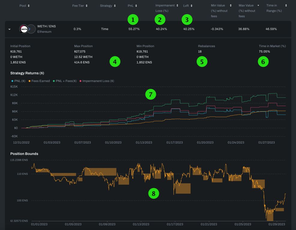
(1) PnL
The overall profit is derived from the accrued fees and changes in asset valuation.
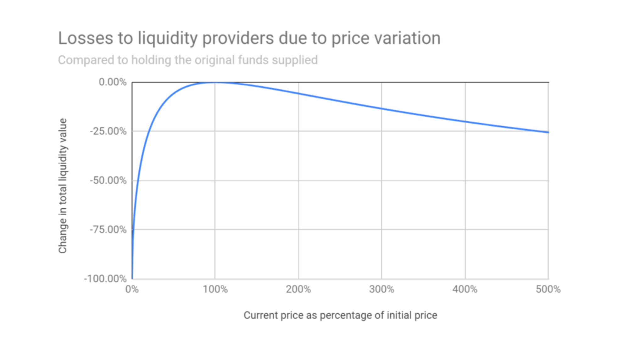
(2) Impermanent Loss
Impermanent loss is the opportunity cost of buying and holding assets. It happens when the value of tokens in a liquidity pool changes compared to when they were initially deposited. Liquidity providers (LPs) may incur losses if the price of one token in the pool diverges significantly from the other token. This risk is inherent in providing liquidity for volatile or asymmetrically valued token pairs.
source: https://tokentuesdays.substack.com/p/eliminating-impermanent-loss
As the diagram illustrates, a 100% Impermanent Loss situation can transpire if the valuation of either asset within the LP plummets to zero.
(3) LvR
While Impermanent Loss is a renowned benchmark metric for Liquidity Provisioning, it has inherent limitations. As previously delineated, a market maker's Impermanent Loss registers at 0% if the price ratio of the assets remains or reverts to its initial value, specifically at the time when liquidity was first provided. This fails to account for price volatility. Consider the scenario of providing liquidity for an ETH/BTC LP. Despite the fluctuation of the price ratio over time, upon your withdrawal, the ratio has reverted to its original value. During the course of your liquidity provisioning, significant arbitrage events have transpired within the LP. While you have accrued swap fees from these transactions, you were concurrently selling your assets for a lesser value than their true worth. Even though your Impermanent Loss stands at 0%, it is logical to surmise that you may have been more profitable as the arbitrager rather than the liquidity provider.
This is precisely where the Loss vs. Rebalancing (LVR) metric comes into consideration. LVR is a metric that juxtaposes the value of your assets in an LP with the value of holding and periodically rebalances the same assets outside the LP in accordance with changes in the price ratio. Essentially, LVR captures the peak profit that can be extracted through arbitrage. Let's delve into an illustrative example of LVR as provided in the linked video:
Visualize an LP holding 1 ETH and 1,000 USDC. The price of ETH escalates to 4,000 USDC, and after arbitrage transactions, the LP now houses 0.5 ETH and 2,000 USDC. This signifies that the market maker effectively traded 0.5 ETH for 1,000 USDC. Consequently, the LP's liquidity stands at $4,000. Now, with LVR in mind, envision a trader possessing 1 ETH and 1,000 USDC in their personal wallet. Observing the LP rebalancing via the effective sale of 0.5 ETH for USDC, the trader follows suit and sells 0.5 ETH for 2,000 USDC in an external market (e.g., a centralized exchange). The trader now owns 0.5 ETH and 3,000 USDC, resulting in an asset value of $5,000 as opposed to the LP's $4,000. The difference of $1,000 stands as the LVR.
Contrasting with IL, each transaction within an LP incurs some degree of LVR. This facilitates the plotting of requisite trading fees as a function of the asset's volatility and the pool’s liquidity. For example, in Uniswap v2, the function is where sigma is the daily volatility of the LP’s price and f is the pool fee in BPS. Consequently, an LP with a daily volatility of 5% and a fee of 30 BPS necessitates roughly 10.4% of the LP’s liquidity in daily trading volume to achieve a break-even point with LVR.
The calculation of LvR (Leverage Ratio) occurs only once per period for a position that is evenly balanced. It remains consistent across different price sentiments and is not altered based on varying sentiments. Consequently, when considering the same pool and period, the LvR value will be identical for simulations involving Positive, Neutral, and Negative price sentiments.
NOTE: The main metric that is comparable across pools is the strategy PnL. LVR and IL are not good comparisons between pools; only after fees. A pool that has a higher LVR than another might have hugely larger fees, thus making it seem better, despite the fact that it has more LVR
(4) Strategy Volatility
This section provides insights into the minimum and maximum value of the portfolio throughout the simulation. By examining this data, users can gain a deeper understanding of the volatility of the portfolio value and determine whether it aligns with their risk appetite.
(5) Number of Position Rebalancing Events
The number of rebalancing events offers a quick overview of the expected transaction fees. Since transaction fees can vary significantly, and different users may value transaction costs differently, the number of rebalancing actions provides a valuable measure for users to assess transaction fees.
(6) Time In Market
A standard metric in Market Making is the percentage of time liquidity is provided.
(7) Strategy Returns
An interactive graph is available to show the evolution of profit and loss (PnL) throughout the simulation. This graph offers a visualization of the PnL components, including asset value and fees, as well as impermanent loss, which can be helpful in assessing the PnL.
(8) Position Bounds
An interactive graph displays the Base Asset price over the simulation and the position bounds at each point in time. This provides a holistic view of the asset price, along with the market-making activity and reactions to changes in volatility.