Gearbox LT Methodology
Summary
This methodology proposes a framework to derive liquidation thresholds (LT) and liquidation bonuses (LB) specifically for LSTs and LRTs on Gearbox, which are assets closely related to ETH. These tokens are fundamentally priced on Gearbox based on their intrinsic value as receipt tokens representing underlying staked or restaked ETH, when withdrawals are enabled. However, during periods of significant market volatility, LSTs and LRTs may temporarily deviate from their fundamental ETH value in the open market due to factors such as liquidity constraints, market sentiment, and liquidation events.
With the Gearbox protocol transitioning to fundamental oracles, these market deviations, though temporary, can create arbitrage opportunities if the deviation persists beyond a certain threshold. To address this, the framework includes a circuit breaker mechanism designed to mitigate such arbitrage by temporarily pausing the market during significant deviations. This prevents exploitative behavior during large market drawdowns. While this exploitative behavior does not expose Gearbox to bad debt, it comes at the cost of liquidity providers.
The framework leverages a correlated, mean-reverting GARCH model where the first process models the price of ETH, and the second process models the price of LSTs/LRTs. This model helps in understanding and predicting the volatility and correlation between these assets, which is crucial for setting appropriate LTs and LBs. Additionally, the framework considers design constraints such as the availability of partial liquidations under specified LTs. It also allows for the protocol to tailor parameters according to the specific collateral asset used and its corresponding debt counterpart, thereby effectively managing and isolating generalized risks. This approach ensures that the protocol remains resilient and adaptable to different market conditions while safeguarding against potential systemic risks.
Motivation
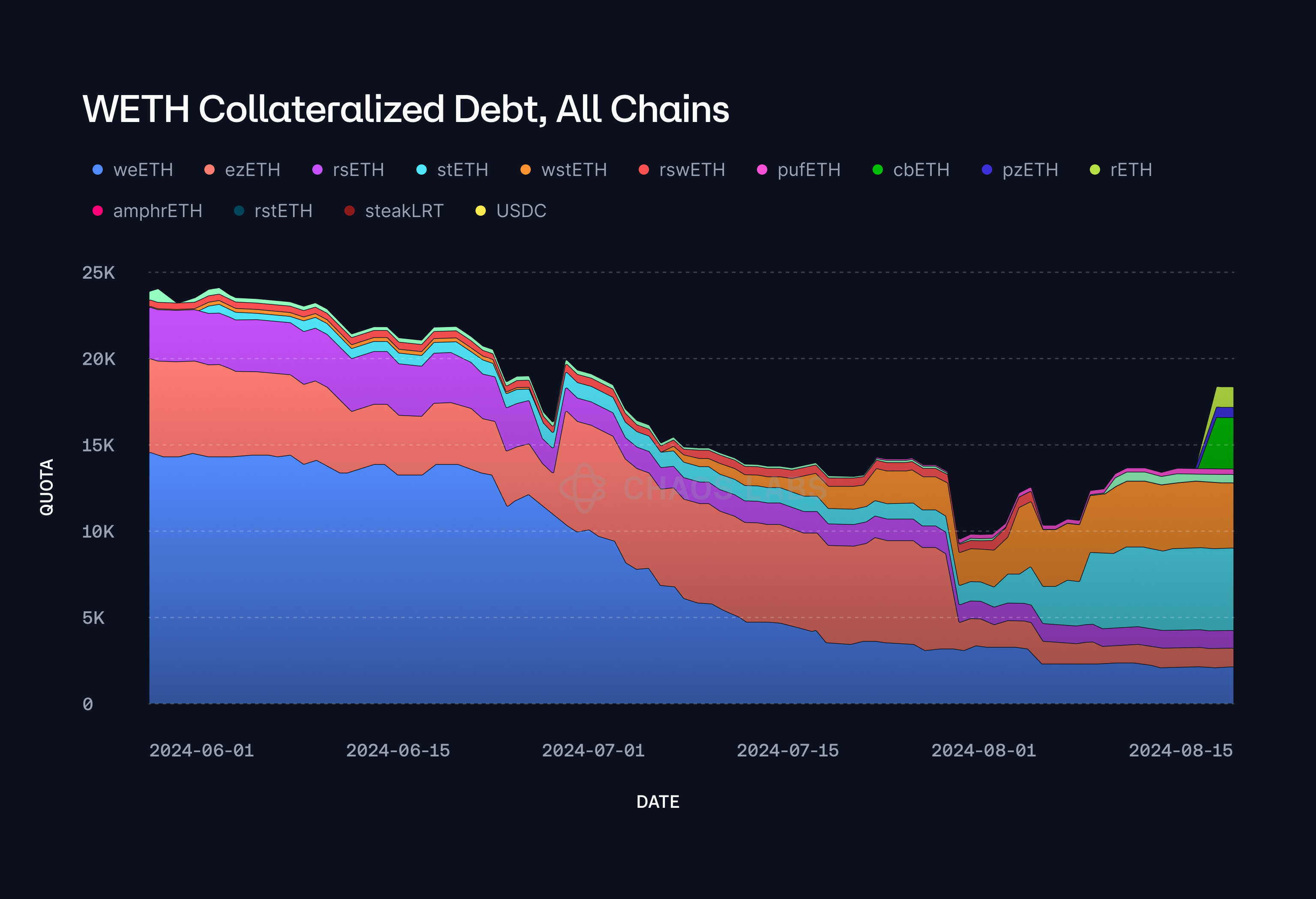
Historically, all of Gearbox’s WETH-denominated debt has been associated with collateral assets that are highly correlated with WETH, as is evident in the accompanying plot. This significant correlation between collateral and debt has largely defined the protocol's risk dynamics and informed its approach to managing market fluctuations and liquidation strategies.
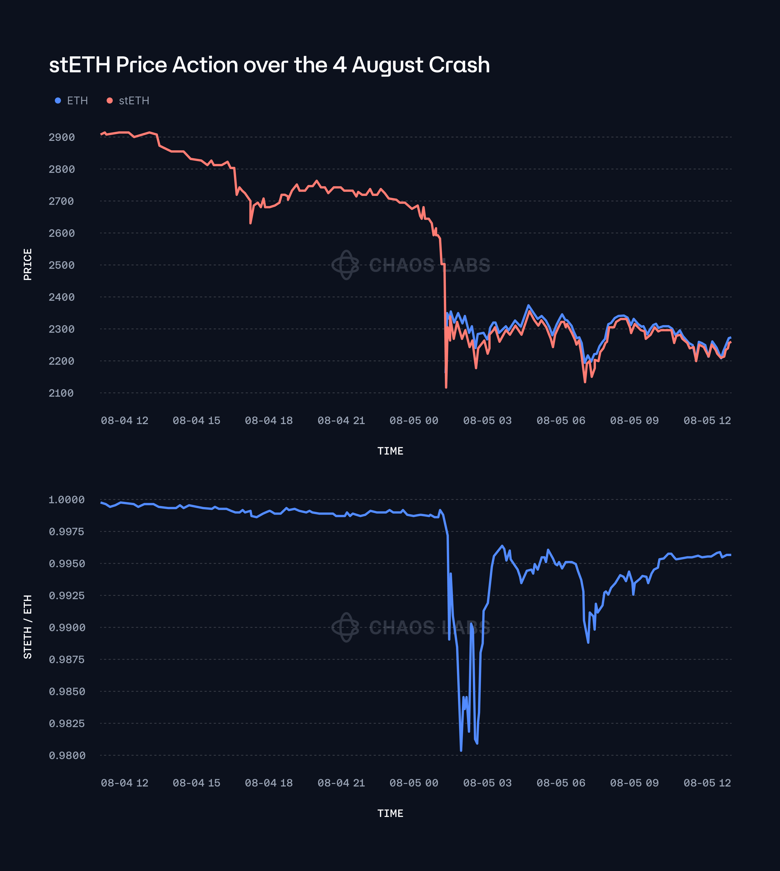
However, with the recent shift towards utilizing fundamental oracles, there is an increased potential for market price deviations from the underlying fundamental values of these correlated assets. Such deviations can lead to a global mispricing across the protocol, introducing new risks that must be carefully managed. For instance, during the most recent market downturn, the underlying market price of stETH temporarily dropped to 0.98 relative to ETH for approximately 30 minutes before gradually reverting to its expected value. This incident is depicted in the plot below, highlighting the transient nature of such deviations and its mean-reverting tendencies.
With the ability to isolate parameters based on the specific collateral-debt asset pairings, the protocol can optimally calibrate responses to price deviations according to the volatility characteristics of each underlying collateral relative to its corresponding debt asset. If the LST/LRT market price relative to its fundamental value falls below the predefined LT, one of the two PausableAdmins can set its quota to 0 by invoking the forbidToken function. This pause serves to prevent users from exploiting a mispriced oracle during periods of significant market deviation, under the assumption that the market price will revert back to its fundamental value in time. By implementing this safeguard, the protocol aims to preserve market integrity and protect against potential arbitrage activities that could lead to destabilization, such as artificially elevated utilization rates and interest spikes.
Model Specification
Modeling the Price of ETH Using a GARCH(1,1) Process
The modeling of the price dynamics of ETH is predicated upon capturing the inherent volatility clustering commonly observed in financial time series. Volatility clustering is the phenomenon where periods of high volatility tend to be followed by high volatility, and periods of low volatility tend to follow low volatility. To model these dynamics, we employ the Generalized Autoregressive Conditional Heteroskedasticity (GARCH) model, specifically a GARCH(1,1) process, which has proven to be effective in modeling such characteristics in financial data.
The process is defined as follows:
Log-Return of ETH
Where:
- denotes the log-return of the ETH price at time t.
- represents the constant mean of the return process, reflecting the average return over time.
- is the innovation term at time t, encapsulating the unexpected component or shock to the return.
Innovation Term and Its Relation to Volatility:
Where:
- denotes the conditional standard deviation of the return at time t, capturing the dynamic nature of volatility.
- represents a standard normal random variable,
- introducing the stochastic element into the model.
Conditional Variance Equation:
Where:
- represents the conditional variance (squared volatility) at time t.
- is a constant term, representing the long-run average level of variance.
- is the coefficient for the lagged squared innovation,
- capturing the immediate impact of past shocks on current volatility.
- is the coefficient for the lagged conditional variance,
- which reflects the persistence of volatility over time.
The parameters
are estimated using maximum likelihood estimation (MLE) based on historical log-return data for ETH. The GARCH(1,1) model effectively captures the volatility dynamics by allowing the conditional variance to evolve over time in response to past innovations and past variance levels.
Modeling the Price of LST/LRT Using a Mean-Reverting Process
The price dynamics of LSTs and LRTs are modeled using a mean-reverting process. The rationale behind employing a mean-reverting model stems from the expectation that the prices of these tokens tend to revert towards a fundamental value or parity with ETH over time. This characteristic is particularly pertinent to LSTs/LRTs, as they are derivatives or representations of staked ETH, and thus, their prices should not deviate significantly from the price of ETH over the long term due to the available arbitrage against the primary market.
The mean-reverting process is defined as follows:
Mean-Reverting Process:
Where:
- denotes the log-return of the LST/LRT price at time t.
- represents the log-return of ETH at time t, serving as the target or equilibrium level to which the LST/LRT price is expected to revert.
- is the mean-reversion coefficient, which quantifies the speed at which the LST/LRT price reverts to the ETH price. A larger value of theta indicates faster reversion.
- is the innovation term at time t, representing the unexpected shock to the LST/LRT price.
The term
reflects the correction towards the target (i.e., ETH price), with the magnitude of the correction being proportional to the deviation of the LST/LRT price from the ETH price in the previous period.
Innovation Term and Its Volatility:
Where:
- denotes the conditional standard deviation of the LST/LRT return at time t.
- represents a standard normal random variable,
- introducing randomness into the model.
Conditional Variance Equation for LST/LRT:
Where:
- represents the conditional variance of the LST/LRT returns at time t.
- is a constant term, representing the long-term average variance level.
- is the coefficient for the lagged squared innovation,
- capturing the effect of past shocks on current volatility.
- is the coefficient for the lagged conditional variance,
- reflecting the persistence of volatility in the LST/LRT returns.
Similar to the ETH model, the parameters
are estimated using historical data on LST/LRT returns.
Modeling the Correlation Between ETH and LST/LRT Price Movements
Given that the price movements of LST/LRT are expected to be closely related to those of ETH, it is essential to model the correlation between the two processes. The correlation structure is introduced by assuming that the innovations
and
are jointly normally distributed (bivariate distributions), as follows:
Where
represents the correlation coefficient between the innovations of the ETH and LST/LRT processes. The introduction of this correlation structure allows the model to account for the simultaneous and related movements of ETH and LST/LRT prices, providing a more realistic depiction of their joint dynamics.
Estimating the Mean-Reversion Parameter
The mean-reversion parameter, theta, plays a crucial role in determining how quickly the LST/LRT price aligns with the ETH price. Estimating this parameter requires reformulating the mean-reversion model into a regression framework, which facilitates the estimation using standard statistical techniques.
The mean-reverting process can be expressed in a linear regression form as follows:
In this equation:
- is the change in the log-return of the LST/LRT price from period t-1 to period t.
- represents the deviation of the ETH log-return from the LST/LRT log-return in the previous period.
- is the coefficient of interest, capturing the speed of mean reversion.
The estimation of theta is conducted using historical data on the returns of ETH and LST/LRT during the recent large market downturn, through ordinary least squares (OLS) regression. A high value of theta would indicate a rapid adjustment of the LST/LRT price towards the ETH price, while a lower value would suggest a slower convergence.
Monte Carlo Simulations for Liquidation Threshold Design
Monte Carlo simulations are employed to assess the risk associated with adverse price deviations between ETH and LST/LRT. The simulations generate a large number of potential future price paths, providing insights into the range of possible outcomes and enabling the design of a robust LT.
Simulating Price Trajectories:
Using the previously estimated GARCH(1,1) model for ETH and the mean-reverting process for LST/LRT, we simulate 10,000 potential price trajectories for both assets. The simulations take into account both the stochastic nature of the innovations and the conditional volatility of returns, ensuring that the generated price paths reflect the complex dynamics observed in the historical data.
Identifying Worst-Case Scenarios:
Among the simulated price paths, particular attention is given to identifying the worst-case scenarios, where the price of LST/LRT deviates significantly from that of ETH. These scenarios represent the potential for adverse outcomes, where the value of LST/LRT could fall to a level that poses a risk to the stability of the protocol.
Designing the Liquidation Threshold:
The worst-case scenarios provide vital insights for optimizing the LT, ensuring it includes a robust buffer between the maximum collateral and debt values based on fundamental pricing. This conservative threshold aims to safeguard the protocol against extreme market conditions, preventing users from exploiting significant mispricings and ensuring the system's resilience.
Simulation Results
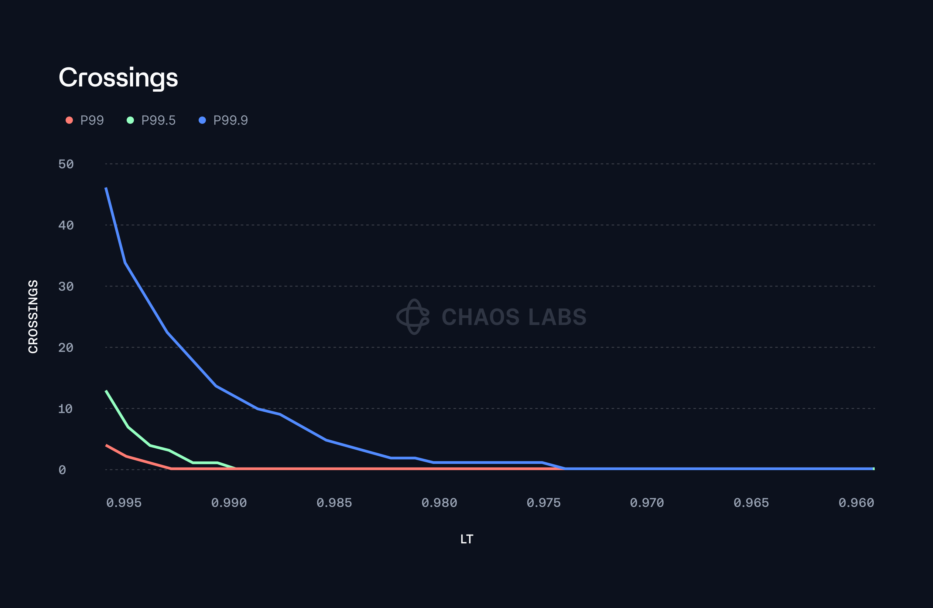
The presented plots provide a detailed analysis of the behavior of stETH when subjected to different LTs using extensive Monte Carlo simulations. These simulations are designed to assess how the stETH/ETH price ratio interacts with these thresholds over numerous potential future price paths, offering insights into the risk dynamics under various market conditions.
The first plot focuses on the frequency with which the stETH/ETH price ratio crosses the defined LT during the simulation period. As the LT becomes more stringent (i.e., a lower LT value), the plot clearly shows a decrease in the number of crossings. This trend is particularly pronounced at higher percentiles, such as P99.9, where the LT is set to be highly conservative. This crossing frequency, however, diminishes exponentially as the threshold continues to decrease, suggesting a non-linear relationship between the LT value and the likelihood of crossing.
The second plot provides a complementary perspective by depicting the total duration, measured in minutes, that the stETH/ETH ratio remains below the LT across all simulated paths. This duration is critical because it acts as an indirect measure of the potential market impact during periods of stress, reflecting how long stETH could potentially be sold at a discount due to the price being below the threshold. The objective is to quantify the expected change in duration that the LT is breached to estimate the impact of the breach for Gearbox. This extended period below the LT suggests that the market could experience prolonged sell pressure over tail events, which could exacerbate the impact on the stETH price during these adverse conditions.
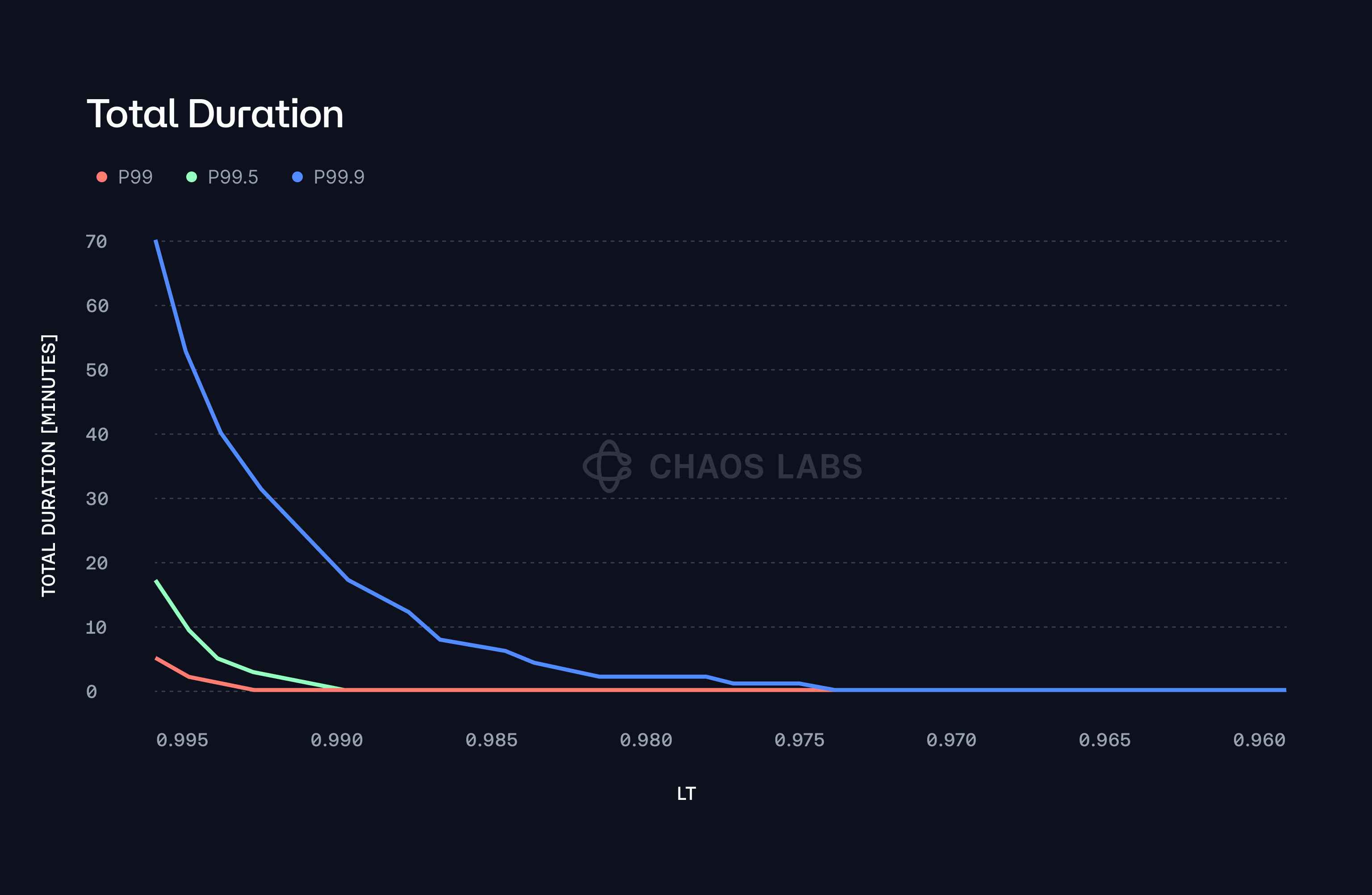
When examining higher percentiles, such as P99.9, the data indicates that these prolonged durations and frequent threshold crossings become even more significant, before zeroing out at a threshold of 97.4%. This is consistent with the intuition that at higher confidence levels, the system must adopt a more conservative stance, resulting in stricter thresholds. These more lenient thresholds are intended to mitigate the risk of deviations by triggering protective measures earlier, yet the trade-off is that they also lead to more frequent and extended periods where the price remains below the threshold. This phenomenon underscores the importance of selecting an appropriate LT that balances the need for frequent intervention (to protect the system) with the risk of extended adverse price deviations that could lead to market instability.
Partial Liquidation Considerations
Over recent months, Gearbox has strategically implemented and whitelisted a partial liquidator bot as a proactive measure to address the challenges inherent in the liquidation process, particularly the significant selling pressure and profitability constraints that are often encountered during full liquidations of credit accounts. The introduction of partial liquidations represents a nuanced approach, designed to mitigate these issues by allowing for more controlled and less disruptive liquidations. However, these partial liquidations come with a critical constraint: the liquidated position must be restored to a health factor above 1. This requirement ensures that, following the liquidation event, the credit account returns to a state of financial stability and is no longer at immediate risk of further liquidation.
The precise percentage of the credit account's debt that must be repaid to achieve this healthy state, given a particular LT, is governed by the following equation:
where:
- represents the initial health factor of the position prior to liquidation. This value reflects the ratio of the account's collateral to its debt, normalized by the LT, providing an indication of the account's risk level before the liquidation process begins.
- LP refers to the liquidation discount, which is calculated as 1 − bonus. This discount is the reduction applied to the value of the collateral being liquidated, typically incentivizing liquidators by allowing them to purchase the collateral at a price below its market value.
- LF stands for the liquidation fee, which is a fee paid to the protocol during the liquidation process. This fee is deducted from the collateral or debt and is designed to cover the costs associated with executing the liquidation.
The heatmap provided visually captures the intricate relationship between the LT, the health factor at the point of liquidation
, and the percentage of debt that must be repaid to restore the position to a healthy state, as defined by the parameters currently in use within the Restaking WETH Credit Manager. As both the LT and the health factor increase, the heatmap transitions from lower percentages (represented by purple hues) to higher percentages (represented by yellow hues). This gradient reflects the increasing proportion of debt that must be repaid to achieve the necessary health factor.
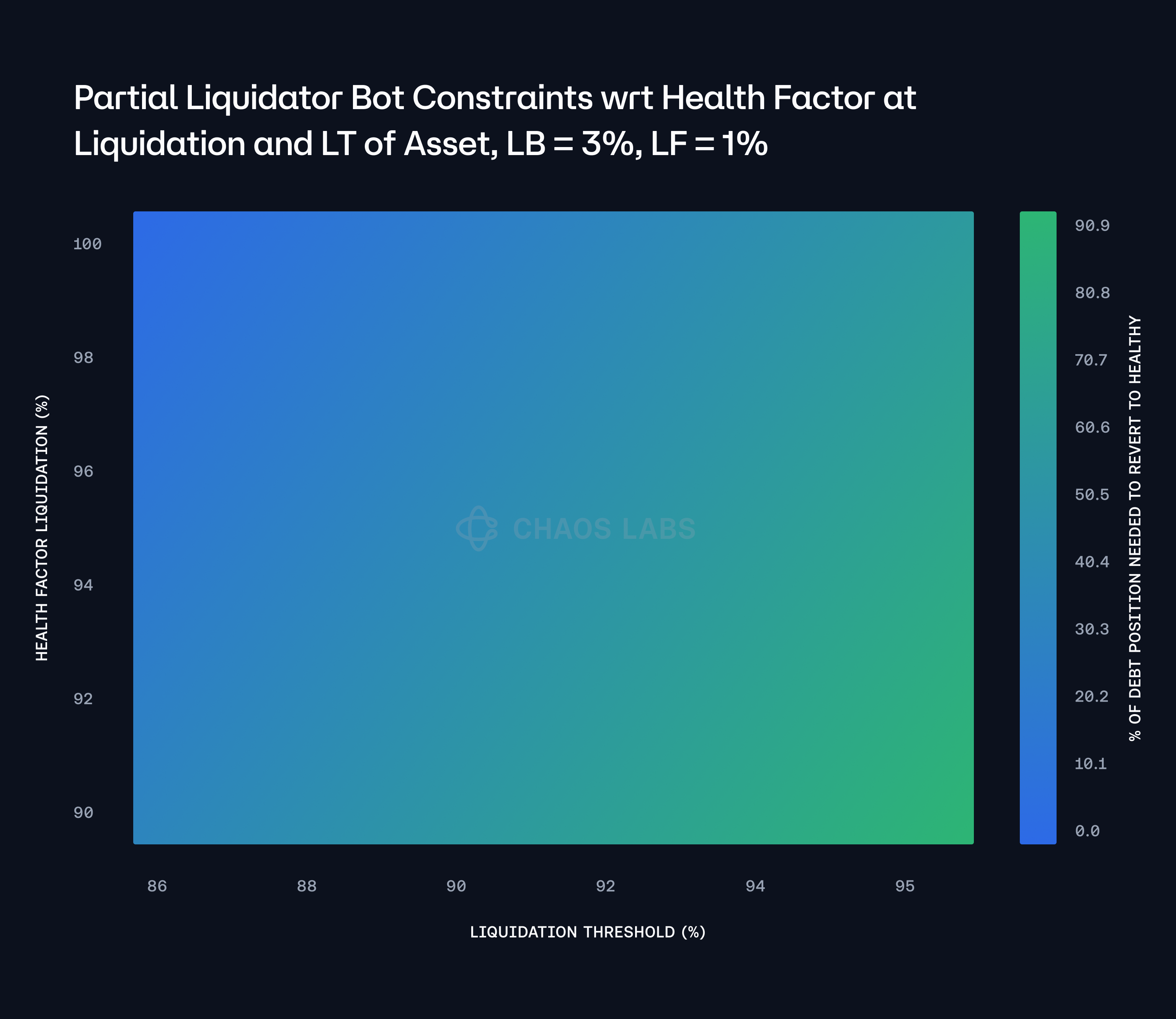
The visualization clearly illustrates that higher LT and health factors necessitate more substantial debt repayments to restore the account to a healthy state. This finding underscores the impact of liquidation policy decisions on the required debt adjustments during partial liquidations. As the health factor worsens, the amount of debt that needs to be repaid increases significantly, highlighting the complexity and sensitivity of this multidimensional optimization problem. The underlying market parameters and the aggregate behavior of these variables introduce additional layers of complexity, making it crucial to carefully consider the implications of different liquidation policies.
Liquidations with Fundamental Oracles and Correlated Debt: Optimizing LT/LB
As mentioned previously, in scenarios where significant deviations in the market price of a correlated asset occur, the protocol has designed an enshrined circuit breaker mechanism to manage these fluctuations.
However, it is essential to consider a worst-case scenario—one where there is no extreme slashing event (whereby the fundamental value will decrease accordingly), and WETH interest rates surpass the effective growth rate of the LST or LRT over an extended period. In such a scenario, and assuming the credit account has not been manually closed due to unprofitability, the debt position could gradually become unprofitable as the Loan-to-Value (LTV) ratio of the credit account slowly increases, drawing closer to the LT. As the LTV ratio approaches this threshold, the protocol would effectively obtain a sufficient time buffer to prevent the accrual of bad debt or to allow for the triggering of partial liquidations, given by the gradual growth in the LTV.
The underlying assumption in this scenario is that the net market price deviation—after accounting for slippage and fees—remains smaller than the LB. If this condition holds, the debt position will stay profitable for liquidation, meaning that partial liquidations can still occur in relation to the health factor at any given time t, provided that the LT and LB parameters are appropriately set. This profitability criterion is crucial because it determines whether the liquidation process will be successful within the predetermined payoff function for a given liquidator.
The accompanying heatmap offers a detailed visualization of the relationship between the LT, the LB, and the difference in debt valuation at two critical junctures: when a position first becomes eligible for liquidation and when partial liquidations are no longer possible. The heatmap effectively captures the interplay between these variables, highlighting how changes in the LT and the LB can influence the point at which a debt position transitions from being eligible for liquidation to being unable to liquidate partially.
These values, represented within the heatmap, can be linearly interpolated to estimate the minimum percentage of debt that must be repaid (minDebtRepaid%) based on the current market price deviation from the initial point of eligibility. This interpolation provides a practical tool for assessing the risk and determining the necessary actions to maintain the health of the credit account. By understanding these dynamics, the protocol can better manage the liquidation process, ensuring that it remains effective and efficient, even under adverse market conditions.
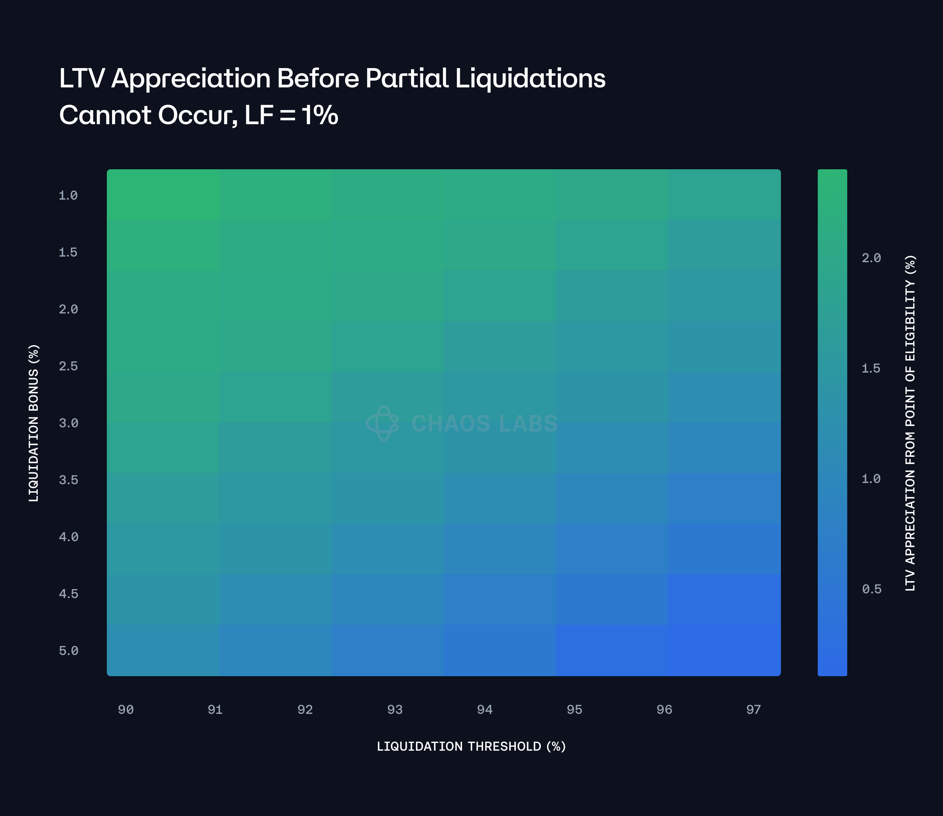
For instance, under a scenario where the LB is set at 1% and the LT is at 97%, the protocol will effectively maintain an approximate 1% net buffer after passing the LT before the position reaches a point where partial liquidations are no longer feasible. This buffer represents the safety margin that allows the position to remain eligible for partial liquidations as the Loan-to-Value (LTV) ratio increases. This scaling process reflects the decreasing profitability of the debt position for liquidation, which eventually leads to a state where partial liquidations can no longer be performed.
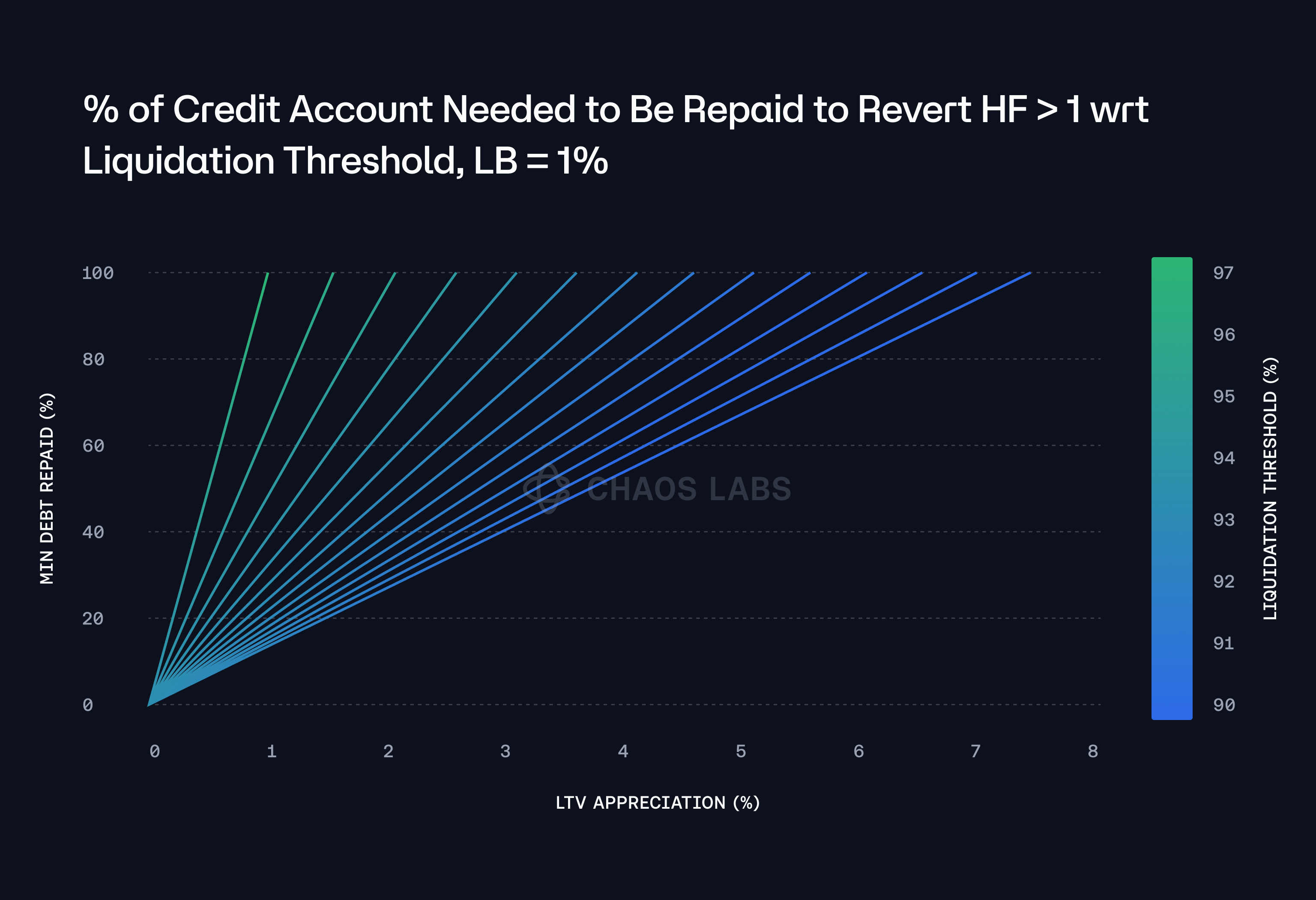
This relationship between the LB, the LT, and the LTV appreciation can be more clearly understood by examining the two-dimensional plot below, which specifically plots the top row of the heatmap. In this plot, the net buffer is represented as a function of the LTV ratio, providing a straightforward visualization of how the buffer shrinks as the LTV ratio increases for a given LT. The plot illustrates the linear nature of this relationship, where the buffer steadily decreases in direct proportion to the rise in the LTV ratio.
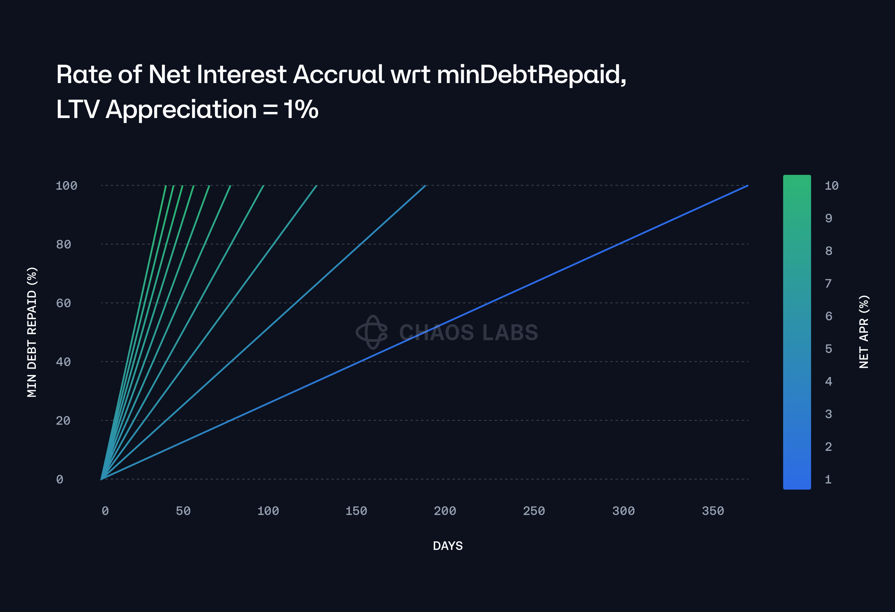
With a 1% 'LTV Appreciation' value, and considering varying net interest accrual (post-staking yield), the partial liquidator bot would have an extended timeframe during which partial liquidations remain feasible. This timeframe significantly exceeds the duration of historical deviations between market price and underlying fundamental value, as illustrated in the plot below.
Conclusion
In scenarios where the collateral asset exhibits a strong correlation with its corresponding debt counterpart, the LB can be finely tuned to a relatively low and stable value in relation to the LT, such as 1%, as seen in other lending protocols such as Aave. This adjustment is predicated on the time-based assumption that the liquidator, when executing partial liquidations on a given position, does so in response to the effective market price deviation of the underlying asset from its intrinsic fundamental value. This deviation tends to remain within a profitable margin nearly 100% of the time. As the LTV ratio of the position increases, this growth is largely gradual, driven by the accrual of net interest over time.
Assuming the LT is parameterized based on market price deviations observed in LSTs and LRTs, especially those with live withdrawal mechanisms, the model is designed to optimize the mitigation of arbitrage opportunities, the frequency of forbidToken events, and the adequate incentivization of liquidators. It also ensures that a sufficient time buffer exists for partial liquidations to occur within the given constraints. As such, the derived LT acts as a proxy for the implied risks associated with the underlying asset from a fundamental perspective, given by the extreme percentiles observed in the historically parameterized market price deviation. By considering these factors, we can accurately parameterize specific LSTs and LRTs backing WETH debt, aligning them with both market dynamics and the asset's risk profile.
Introducing Chaos Oracles: The Next Generation Oracle Protocol
At Chaos Labs, we've always believed that robust risk management and reliable data are the foundations of a thriving DeFi ecosystem. With Edge, we're putting that belief into action, providing a solution that doesn't just report prices but actively contributes to the security and efficiency of on-chain finance.
Oracle Risk and Security Standards: Data Replicability (Pt. 4)
Data replicability is the capacity for third parties to independently recreate an Oracle’s reported prices. This requires transparency into two key components of the Oracle’s system: its data inputs and its aggregation methodology.
Risk Less.
Know More.
Get updates on our research, product, and launch.